Charts, Plots, and Matplotlib

Matplotlib is a widely used library for creating high quality static, animated, and interactive data visualizations. It has a long history within the Python community. Matplotlib’s contributions to the scientific community cannot be overstated. Integrating matplotlib into py5 creates many exciting possibilities.

In the future, matplotlib will have even more integrations with py5, beyond what is discussed here. Stay tuned!

Setup

Install matplotlib with pip or with conda.

pip install matplotlib

conda install matplotlib -c conda-forge

Refer to matplotlib’s Getting Started page or Installation Guide for more information.

Figure Objects

Converting matplotlib Figure objects to Py5Image objects with convert_image() is straightforward but there are important performance considerations that must be addressed to use this feature well.

Example with Performance Problems

Let’s start with an example that has some performance problems. Understanding the performance problems is necessary to show you how to use py5 and matplotlib together optimally. We will work through the performance problems to demonstrate better ways to use py5 and matplotlib in a Sketch.

To begin, we will import matplotlib and some other libraries we will use for our examples.

from collections import deque

import numpy as np
import matplotlib as mpl
import matplotlib.pyplot as plt
from matplotlib.colors import LinearSegmentedColormap

import py5_tools
import py5

Next we will set matplotlib’s drawing style. There are many style sheets to choose from. Here we are using “ggplot” with the “fast” style to improve performance.

We will not use the matplotlib Jupyter Notebook magic %matplotlib inline. It isn’t necessary for this example and it seems to conflict with the code py5 uses to run correctly on macOS.

mpl.style.use(['ggplot', 'fast'])

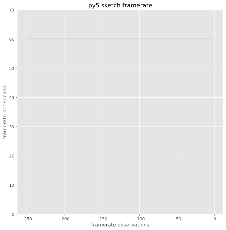
For our example we will create a Sketch that plots its own frame rate. We will collect the frame rate numbers in a special data structure called a “deque”. This data structure will store the most recent 250 frame rate observations. It will do this automatically by removing old values as new values are added. We will also pre-populate the deque with initial values of 60.

frame_rates = deque([60] * 250, maxlen=250)

Next we will create a function for creating our matplotlib chart. As you can see, this is a nice looking chart. New observations are added to the right side of the chart. The data points get successively older as one moves from right to left.

def create_chart(frame_rates):
    figure, ax1 = plt.subplots(1, 1, figsize=(9, 9))
    line, = ax1.plot(range(-len(frame_rates), 0), frame_rates)
    ax1.set_ylim(0, 70)
    ax1.set_xlabel('framerate observations')
    ax1.set_ylabel('framerate per second')
    ax1.set_title('py5 sketch framerate')

    return figure, line


create_chart(frame_rates)

(<Figure size 900x900 with 1 Axes>,
 <matplotlib.lines.Line2D at 0x7f8d73ad0e20>)

Finally, we will set the matplotlib backend to AGG. This backend is non-interactive. It is also faster than the other backends, making it a good choice for our work with py5.

After setting this backend, matplotlib Figures will no longer appear embedded in the notebook like you see for the Figure created above.

mpl.use('agg')

Now, the py5 Sketch. Here, we are creating a new chart in each execution of the draw() method. The Figure object is converted to a Py5Image object using convert_image().

Since each call to draw() creates a new Figure, we must close each figure with plt.close() to control memory usage.

def setup():
    py5.size(950, 950)


def draw():
    frame_rates.append(py5.get_frame_rate())

    figure, _ = create_chart(frame_rates)
    chart = py5.convert_image(figure)
    plt.close(figure)

    py5.background(240)
    py5.image(chart, 25, 25)


py5.run_sketch()

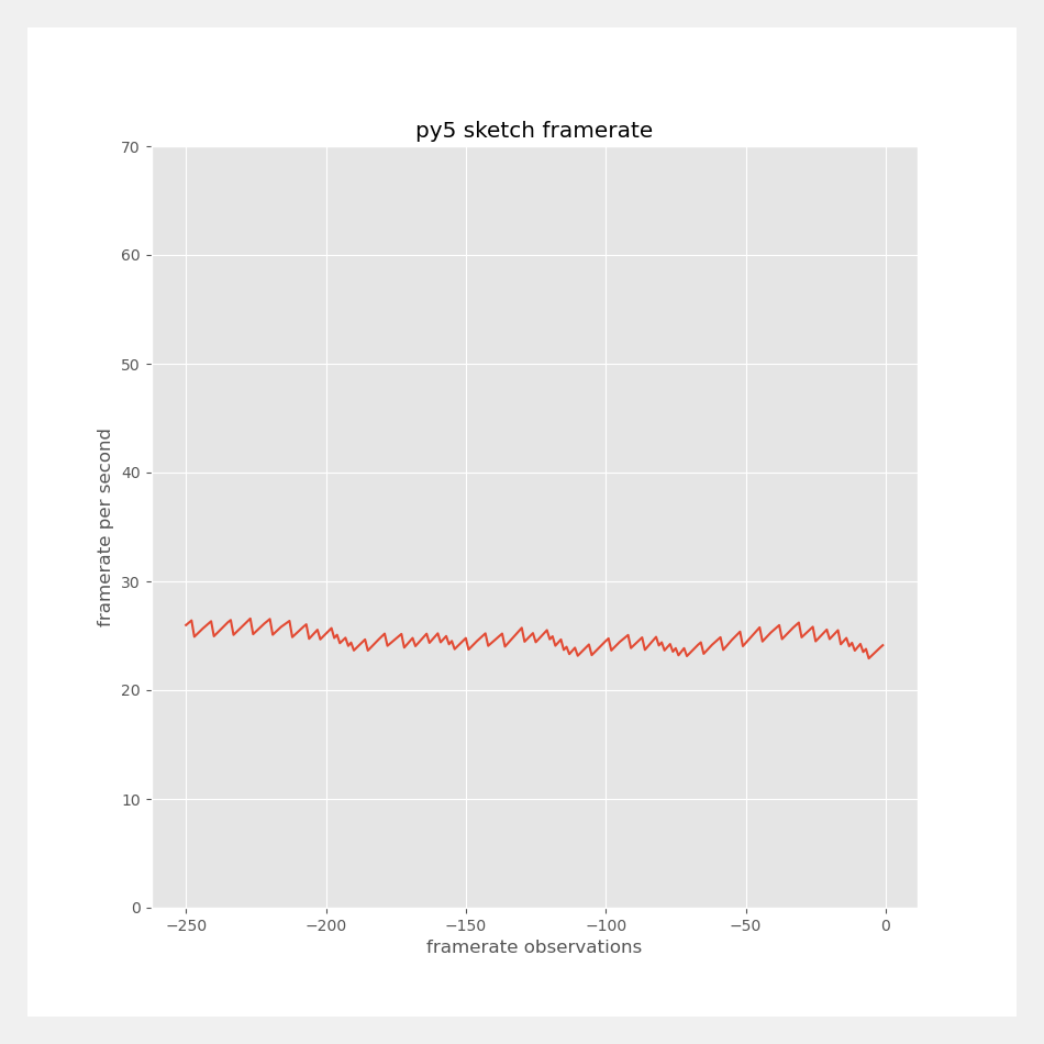
This is slow. We can do better.

py5_tools.screenshot()

Performance Analysis

We will profile the draw() function to investigate why.

py5.profile_draw()

py5.print_line_profiler_stats()

Timer unit: 1e-09 s

Total time: 9.92424 s
File: /tmp/ipykernel_44309/1970811340.py
Function: draw at line 5

Line #      Hits         Time  Per Hit   % Time  Line Contents
==============================================================
     5                                           def draw():
     6       189    1649920.0   8729.7      0.0      frame_rates.append(py5.get_frame_rate())
     7                                           
     8       189 2175164828.0 11508808.6     21.9      figure, _ = create_chart(frame_rates)
     9       188 7278809906.0 38717074.0     73.3      chart = py5.convert_image(figure)
    10       188    4083409.0  21720.3      0.0      plt.close(figure)
    11                                           
    12       188   42502537.0 226077.3      0.4      py5.background(240)
    13       188  422030490.0 2244843.0      4.3      py5.image(chart, 25, 25)

The Sketch is spending the majority of the time in convert_image(). It is also spendng a significant amount of time creating the Figure.

Improved Example

There are a few quick changes we can make to address this.

The first change is to create the Figure one and only one time in setup(). We can then update the Figure’s data with the line’s set_ydata() method. Creating the Figure object once and updating the data is a much more efficient approach. Repeatedly creating matplotlib Figures is in general a bad idea.

The second change is to recycle the Py5Image object. The convert_image() method lets us provide a Py5Image object to write the converted image data into. The Py5Image object must be the correct size. Recycling one Py5Image object in this way lets us skip the repeated object creation of new Py5Image objects and garbage collection of old Py5Image objects.

frame_rates = deque([60] * 250, maxlen=250)


def setup():
    global figure, line, chart
    py5.size(950, 950)

    figure, line = create_chart(frame_rates)
    chart = py5.convert_image(figure)


def draw():
    frame_rates.append(py5.get_frame_rate())

    line.set_ydata(frame_rates)
    py5.convert_image(figure, dst=chart)

    py5.background(240)
    py5.image(chart, 25, 25)


py5.run_sketch()

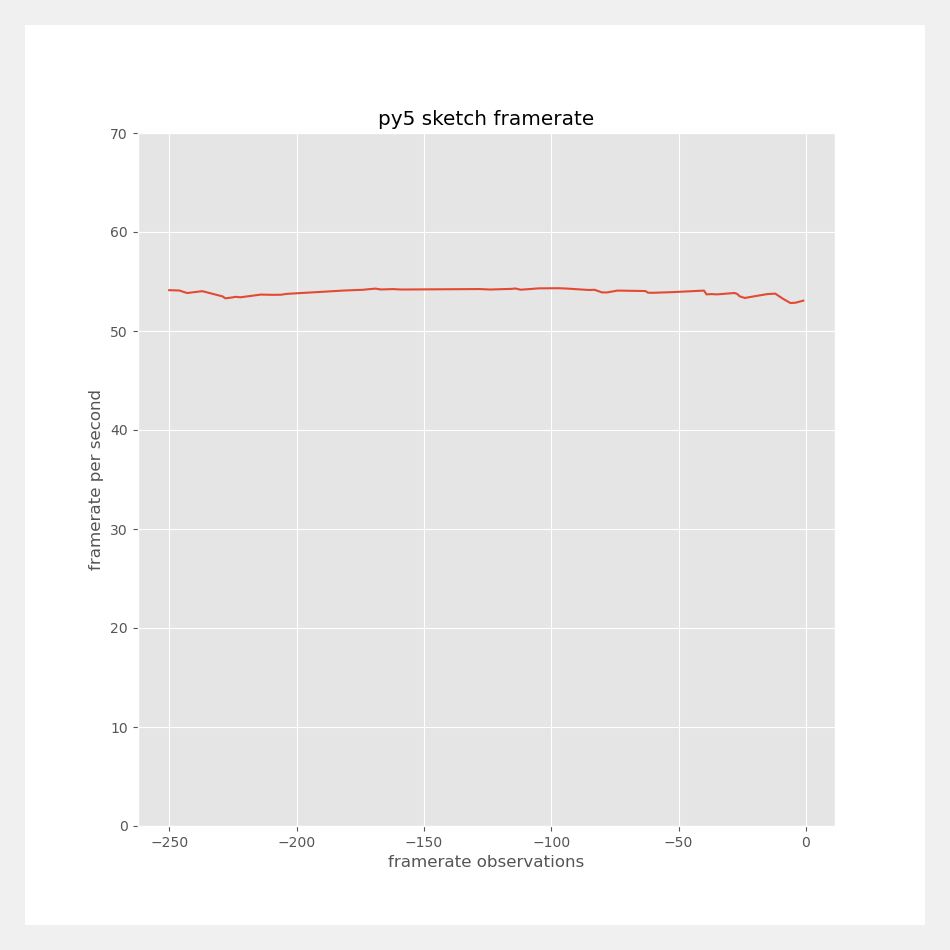
We can see this is significantly faster but still not the Sketch performance we are looking for.

py5_tools.screenshot()

Second Performance Analysis

We can again profile the draw() function to understand why.

py5.profile_draw()

py5.print_line_profiler_stats()

Timer unit: 1e-09 s

Total time: 9.80961 s
File: /tmp/ipykernel_44309/873919406.py
Function: draw at line 12

Line #      Hits         Time  Per Hit   % Time  Line Contents
==============================================================
    12                                           def draw():
    13       437    3037973.0   6951.9      0.0      frame_rates.append(py5.get_frame_rate())
    14                                           
    15       437    6748759.0  15443.4      0.1      line.set_ydata(frame_rates)
    16       436 9337557336.0 21416415.9     95.2      py5.convert_image(figure, dst=chart)
    17                                           
    18       436   68696349.0 157560.4      0.7      py5.background(240)
    19       436  393571112.0 902686.0      4.0      py5.image(chart, 25, 25)

Almost all of the time is spent in convert_image(). The call itself is much faster than before because of the recycled Py5Image object, but if we want to improve the performance of this Sketch, we must figure out how to make it even faster.

Example with Threading

The way to make the Sketch even faster is to move the call to convert_image() out of the draw() function and into a separate thread.

The updated code is below. We will create a new function called update_chart() that will be repeatedly called by launch_repeating_thread().

Moving py5 method calls to a separate thread like this will sometimes have thread-safety issues. A thread safety issue means that code running in two different threads will create a conflict. This can lead to unusual behavior, a programming error, or a crash.

In general, Processing drawing commands are not thread-safe, so calling py5 methods from a thread like this is risky. This is especially true when using the OpenGL renderers P2D and P3D. However, the convert_image() method does not attempt to draw to the screen, so using it in a thread like this is fine.

frame_rates = deque([60] * 250, maxlen=250)


def update_chart(frame_rates, line, figure, chart):
    line.set_ydata(frame_rates)
    py5.convert_image(figure, dst=chart)


def setup():
    global chart
    py5.size(950, 950)

    figure, line = create_chart(frame_rates)
    chart = py5.convert_image(figure)

    py5.launch_repeating_thread(
        update_chart,
        args=(frame_rates, line, figure, chart)
    )


def draw():
    frame_rates.append(py5.get_frame_rate())

    py5.background(240)
    py5.image(chart, 25, 25)


py5.run_sketch()

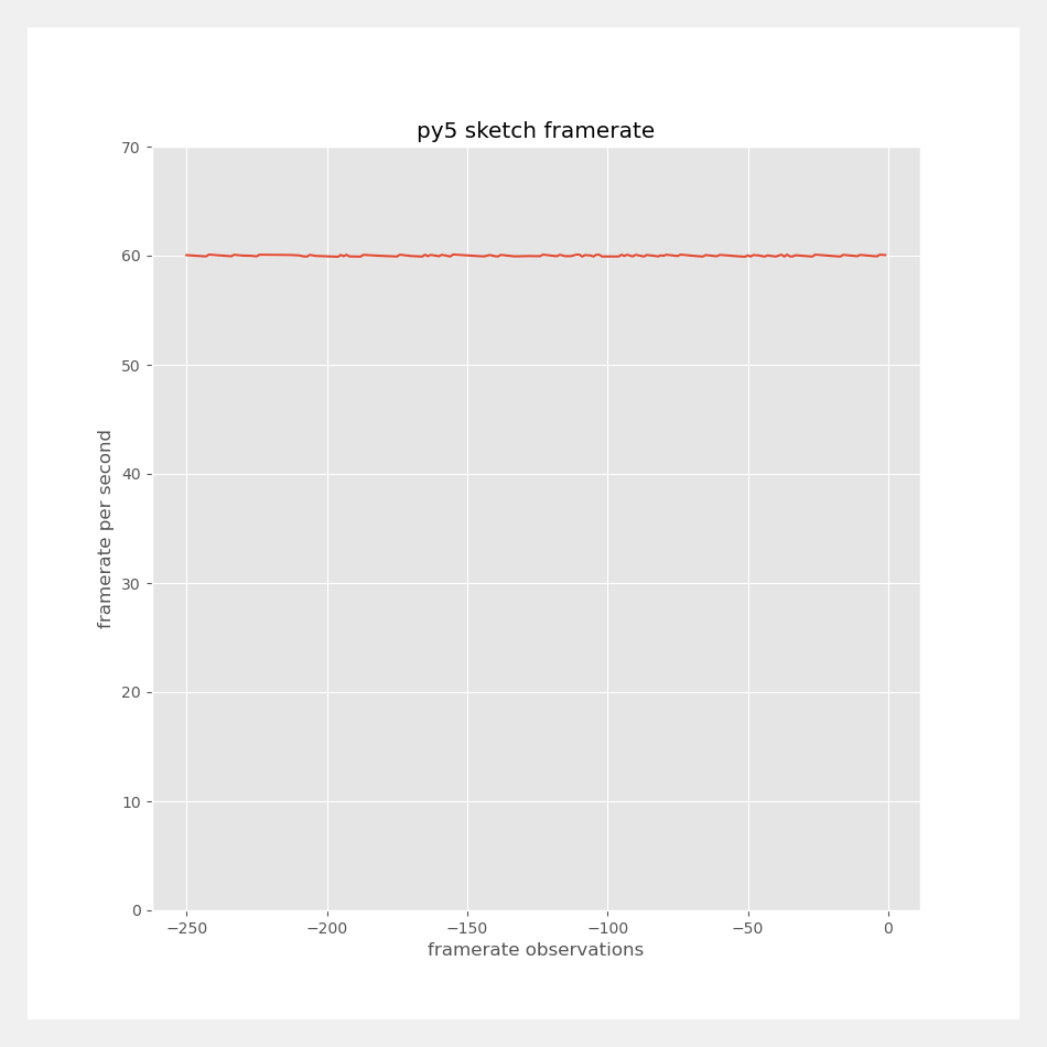
The performance of this new Sketch is now a solid 60 frames per second.

py5_tools.screenshot()

Named Colors

Built in to matplotlib is an extensive list of named colors. Matplotlib users can use this list to customize the aesthetics of their charts. Py5 users can also access this inventory of colors to customize the aesthetics of a Sketch.

Here is a simple example, referencing each color as a string.

def setup():
    py5.size(400, 400)
    py5.background(240)
    py5.no_stroke()

    # matplotlib base color, magenta
    py5.fill('m')
    py5.rect(20, 20, 170, 170)

    # CSS4 colors
    py5.fill('chartreuse')
    py5.rect(20, 210, 170, 170)

    # tableau palette
    py5.fill('tab:orange')
    py5.rect(210, 20, 170, 170)

    # xkcd color survey
    py5.fill('xkcd:blue with a hint of purple')
    py5.rect(210, 210, 170, 170)

    # add some text labels
    py5.fill('black')
    py5.text('m', 70, 105)
    py5.text('chartreuse', 70, 295)
    py5.text('tab:orange', 255, 105)
    py5.text('xkcd:blue with a hint of purple', 220, 295)


py5.run_sketch()

py5_tools.screenshot()

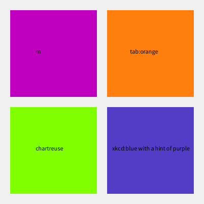
This works well, but it requires you to either remember the names of the available colors or to constantly refer back to the list of named colors. This is an extra challenge for non-english speakers, as well as anyone who cannot remember the correct spelling of words like “chartreuse.”

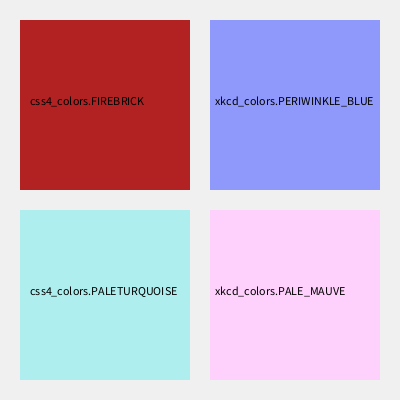
As an alternative, py5 has a built-in dictionary of the full CSS4 and xkcd color survey inventories available for your use. Access the dictionaries with py5.css4_colors and py5.xkcd_colors. These are especially useful when coding an environment that supports code completion, such as Jupyter Notebooks or VSCode. Coders will be able to scroll through the list of color names and select the one that sounds appropriate for their use case.

def setup():
    py5.size(400, 400)
    py5.background(240)
    py5.no_stroke()

    py5.fill(py5.css4_colors.FIREBRICK)
    py5.rect(20, 20, 170, 170)

    py5.fill(py5.css4_colors.PALETURQUOISE)
    py5.rect(20, 210, 170, 170)

    py5.fill(py5.xkcd_colors.PERIWINKLE_BLUE)
    py5.rect(210, 20, 170, 170)

    py5.fill(py5.xkcd_colors.PALE_MAUVE)
    py5.rect(210, 210, 170, 170)

    # add some text labels
    py5.fill(py5.css4_colors.BLACK)
    py5.text('css4_colors.FIREBRICK', 30, 105)
    py5.text('css4_colors.PALETURQUOISE', 30, 295)
    py5.text('xkcd_colors.PERIWINKLE_BLUE', 215, 105)
    py5.text('xkcd_colors.PALE_MAUVE', 215, 295)


py5.run_sketch()

py5_tools.screenshot()

This final color dictionary feature is added to py5 when py5 is built so you can use it without installing matplotlib.

Colormap Color Mode

Processing has two built-in color modes: RGB (red, green, blue) and HSB (hue, saturation, brightness). Py5 adds a third: CMAP, short for colormap.

The main idea behind the Colormap Color Mode is the automatic mapping of values to the colors of a matplotlib colormap palette. This includes support for the colormap’s bad (np.nan) and outlier values.

You will enable the Colormap Color Mode with a call to color_mode(). You can find the list of built-in colormaps in matplotlib’s Colormap reference. The scientific community has done extensive research on colormaps and data visualization. Matplotlib’s documentation provides some insight into how to choose colormaps for your use case.

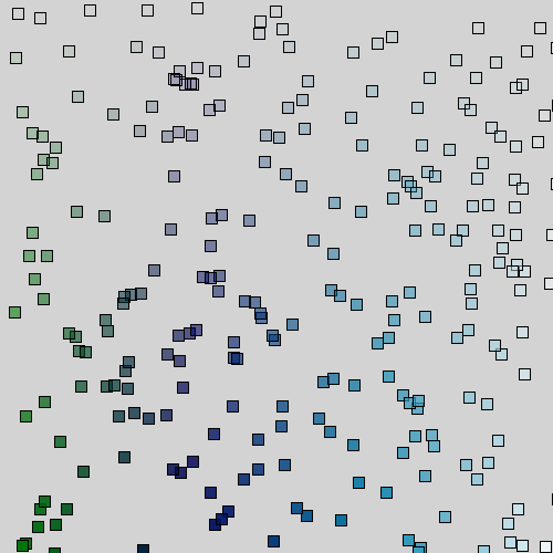
The below example uses the “ocean” colormap with the color range from 0 to the sketch width (500) and the alpha value range from 0 to the sketch height (also 500).

def setup():
    py5.size(500, 500)

    py5.color_mode(py5.CMAP, py5.mpl_cmaps.OCEAN, py5.width, py5.height)

    # bypass the colormap functionality with a named color
    py5.background(py5.css4_colors.LIGHTGRAY)

    for _ in range(250):
        x = py5.random(py5.width)
        y = py5.random(py5.height)
        # fill color determined by x
        # transparency determined by y
        py5.fill(x, y)
        py5.rect(x, y, 10, 10)


py5.run_sketch()

The above example used py5.mpl_cmaps, py5’s built-in dictionary of matplotlib provided Colormaps. We could have just as easily used the string “ocean” there, but like named colors, it is easier to not have to remember the list of available Colormap names.

Observe the call to py5.background(), which uses a named color. Non-numeric values will bypass the Colormap functionality.

Here’s a screenshot of what this example looks like. As you can see, the colors blend from left to right and the transparency varies from top to bottom.

py5_tools.screenshot()

Creating Colormaps

You are not limited to matplotlib’s built-in colormaps. If you like, you can pass color_mode() a matplotlib Colormap object from one of matplotlib’s 3rd party libraries or a Colormap object you create yourself.

Matplotlib provides extensive documentation on how to create your own Colormap. For fun, let’s create a simple one here.

colors = [py5.xkcd_colors.RICH_BLUE,
          py5.xkcd_colors.LIGHT_BLUE,
          py5.xkcd_colors.BRIGHT_RED,
          py5.xkcd_colors.BRIGHT_RED]
nodes = [0.0, 0.5, 0.75, 1.0]

py5_colormap = LinearSegmentedColormap.from_list(
    'py5 example colormap',
    list(zip(nodes, colors))
)

py5_colormap

py5 example colormap

under

bad

over

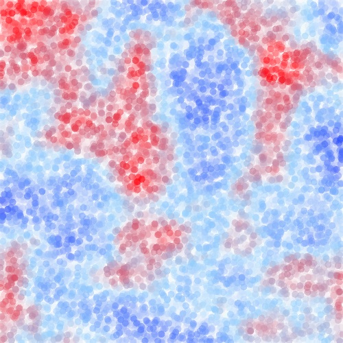
We will use our new Colormap object in a Sketch that draws random points to the screen. The color of each point will be noise values passed through our Colormap.

def setup():
    py5.size(500, 500, py5.P2D)
    py5.color_mode(py5.CMAP, py5_colormap)


def draw():
    py5.no_stroke()
    py5.fill(py5.css4_colors.WHITE, 16)
    py5.rect(0, 0, py5.width, py5.height)

    py5.stroke_weight(10)
    for _ in range(500):
        x = py5.random(py5.width)
        y = py5.random(py5.height)
        val = py5.noise(x / 100, y / 100)
        py5.stroke(val, 128)
        py5.point(x, y)


py5.run_sketch()

In this example, we didn’t pass range values to color_mode(), so the range defaults to 1.0 for the grayscale values and 255 for the alpha values.

Here’s a screenshot of what this looks like, with the noise high-points clearly in red.

py5_tools.screenshot()

Function Signatures

Since this is a new feature, we should clearly articulate the function signatures and some details about how all of this works.

The color_mode() reference documentation provides this signature:

color_mode(
    colormap_mode: int,  # CMAP, activating matplotlib Colormap mode
    color_map: Union[str, matplotlib.colors.Colormap],  # name of builtin matplotlib Colormap
    max_map: float,  # range for the color map
    max_a: float,  # range for the alpha
    /,
) -> None

The first parameter will be CMAP and the second parameter will be the name of one of the built-in matplotlib Colormaps or an actual matplotlib.colors.Colormap instance. The third parameter sets the value of the maximum input range; the minimum is always zero. The last parameter sets the value of the maximum alpha value, and works just like the other color modes. The third and fourth parameters are optional and default to 1.0 and 255, respectively.

In our first example, we used this code:

def setup():
    py5.size(500, 500)

    py5.color_mode(py5.CMAP, py5.mpl_cmaps.OCEAN, py5.width, py5.height)

The max_map and max_a values are both 500.

If we then set the stroke style property with py5.stroke(42), py5 would divide the input value 42 by 500 and pass the result into the Colormap. The color value and alpha value would be set by the output of the Colormap. If we set the stroke style property with py5.stroke(42, 250), py5 would get the same color value from the Colormap but override the alpha value to be 250 divided by 500.

You can bypass the colormap functionality by passing a non-numeric argument such as a named color or a color hex code. Refer to All About Colors for more possibilities.

When this color mode is activated, py5 will accept np.nan values and map them to the Colormap’s “bad” or invalid color setting. Typically this is completely transparent. If this isn’t what you want, the best choice is to create your own Colormap and use the instance’s set_bad() method. You can also set a new “bad” value for a built-in Colormap.

This Colormap Color Mode feature does not work for Py5Graphics or Py5Shape objects. It is only available for your Sketch. This shouldn’t limit you in any way because you can always use the Sketch’s color() method as a work-around (i.e. shape.fill(py5.color(42))).